TL;DR
- I implemented Trung’s idea of using kernel methods for safety steering: fit an RBF kernel PCA to benign activations to learn the benign manifold, then use distance from that manifold as a steering gate. I call it KernelSteer.
- This replaces the null-space projection in AlphaSteer, which assumes benign activations occupy a linear subspace. We instead assume they lie on a nonlinear manifold.
- The non-parametric nature of KernelSteer results in a manifold that is tightly coupled to its training data, making it worse on unseen, out of distribution samples compared to AlphaSteer.
Method
Overview
Let h \in \mathbb{R}^d be the residual-stream activation at the last prompt token, read at each steered layer \ell \in L. The intervention is
with two learned components: a gate g(h) \in [0,1] deciding how much to steer this particular prompt, and a unit-norm refusal direction r deciding what to add. The \alpha is the steering strength which is swept.
The benign manifold (the gate)
The RBF kernel over activations is
where \Phi is the implicit feature into an infinite-dimensional space.
The bandwidth \gamma is set by the median heuristic with one scale hyperparameter s:
Given N benign training activations, we form the Gram matrix K_{ij} = k(h_i, h_j), run kernel PCA and keep the top n principal components, written V. Their span is our model of the benign manifold in feature space.
Membership is scored by the reconstruction error
the squared feature-space distance from the benign subspace, computable using the kernel trick. On-manifold prompts have low error; anything the manifold cannot express has high error.
To turn e into a gate we hold out a subset of the benign pool for calibration: let q_b be the median error of the held-out benign calibration activations and q_h the median error of the harmful training activations. Then
so the typical benign prompt maps to 0 and the typical harmful prompt to 1.[1]
The gate values are used to determine the number of principal components n: we choose the n that maximizes the AUC-ROC between the benign calibration errors and the harmful training errors.
Nyström approximation
Exact KPCA needs an eigendecomposition of the N \times N Gram which can quickly become intractable as N gets large (O(N^3)). Instead, we use the Nyström method: choose m landmarks from the benign pool and build features against them only.
Writing k_m(h) = \begin{bmatrix}k(h, z_1), \dots, k(h, z_m)\end{bmatrix} for the kernel values against landmarks z_j, the Nyström feature vector is
where K_{mm} is the landmarks’ own Gram matrix, (K_{mm})_{jl} = k(z_j, z_l). Its inverse square root whitens the landmark basis. And since every RBF feature has unit norm, \lVert \Psi(h) \rVert^2 \le 1 is the fraction of the prompt’s feature energy that is captured by the approximation. Linear PCA on \Psi is kernel PCA restricted to that span, at O(m^2 N + m^3).
The approximation splits the reconstruction error into two parts:
Refusal direction and layer selection
The normalized refusal direction is obtained via diff in means:
Layers are selected as in Jailbreak Antidote: rank every layer by how separable refused vs complied activations are along its r, and steer the top-p fraction. On Llama-3.1-8B this selects 12 layers.
Experiments
For all experiments, I used the OpenSteering benchmark — still a WIP. The benign set includes Alpaca (24,997 examples), and two borderline datasets: OKTest (300) and XSTest (185). For KernelSteer specifically, 20% of the benign set is held out for calibration. The harmful set (8,416 prompts) includes AdvBench (418), JailbreakBench (83), MaliciousInstruct (78), StrongREJECT (245), SorryBench (7,399), the unsafe half of XSTest (152), and HarmBench validation behaviors (41); HarmBench test behaviors, expanded into attack variants by eight attack methods (DirectRequest, GCG, AutoDAN, HumanJailbreaks, ZeroShot, PAIR, TAP, PAP), are reserved for testing. Additionally, malicious prompts are labelled as “refused” or “complied” depending on the specific model’s behavior. In our case, we use this signal for computing r and for selecting layers.
The benchmark measures methods against a pareto front of attack success rate (ASR) for malicious prompts (↓ lower is better), and over-refusal rate (ORR) for benign and borderline prompts (↓). Evaluation uses a held-out test split of every source, subsampled to 64 prompts per source (per attack method for HarmBench); the same subsample is used for every method and every point.
Everything below is on Llama-3.1-8B-Instruct.
First run: the gate protects Alpaca, not the borderline sources
The first attempt at using KernelSteer involved a coefficient sweep on \alpha with reasonable hyperparameters including m=1024 randomly-selected landmarks. Under this configuration, KernelSteer performed far worse than AlphaSteer: higher ORR and ASR. I then investigated the gate values, partitioned by the different benign data sources.
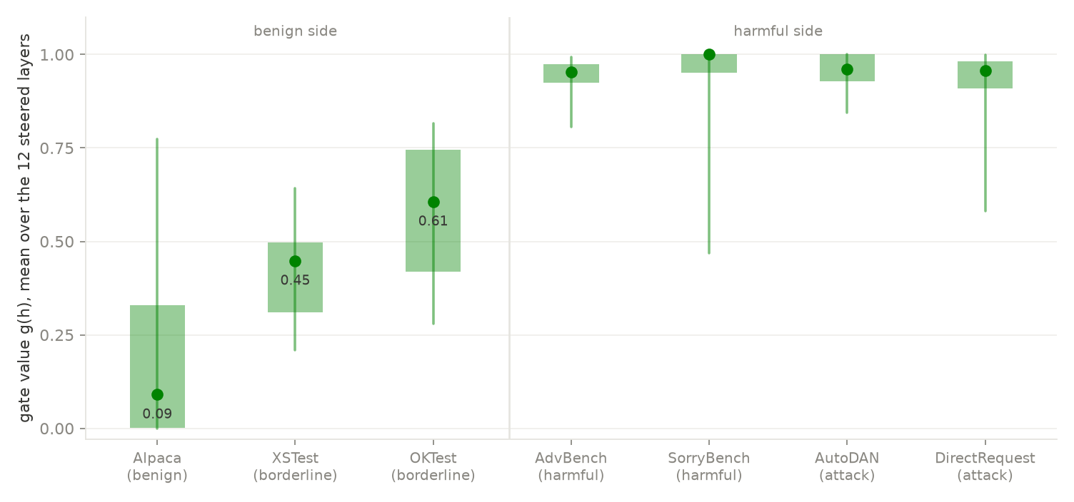
Gate values on held-out test prompts, by source, with randomly-selected landmarks.
This revealed that the gate seemed to be working well for Alpaca, but not for the borderline sources. At this point, I hypothesized that it was because of the landmark selection. Since landmarks are selected randomly, and there are a disproportionate number of Alpaca examples compared to the borderline sources (Alpaca is ~98% of the benign pool), I thought the problem might be that the learned manifold was underrepresenting those borderline sources.
Improving landmark selection
The above finding inspired two alternative landmark selection strategies. The first was stratified sampling — ensuring an equal number of landmarks come from each data source. Using this sampling technique, at \alpha = 0.5, ORR dropped from 0.190 to 0.157 at identical ASR — the improvement coming primarily from better gating for OKTest.
Despite the improvement, stratified sampling has some issues. For example, some data sources might have a broader distribution than others, so they should be assigned more landmarks than a data source consisting of a narrower spread of samples. Quotas also can’t see diversity within a source, and in the real world a benign pool won’t be labelled by source at all. Because of this, I also tried a greedy approach: pivoted-Cholesky max-residual selection. Starting from an empty landmark set, each step picks the prompt whose feature-space representation is currently worst covered — the one with the largest off-subspace energy 1 - \lVert \Psi(x) \rVert^2 with respect to the landmarks chosen so far. This selection strategy was the best performing, however still falls short to AlphaSteer.
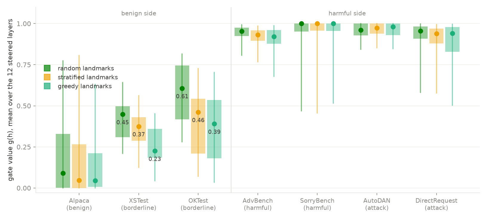
Gate values by source under the three landmark strategies. The borderline medians drop with better coverage (random → stratified → greedy) while Alpaca stays protected and the harmful sources stay caught.
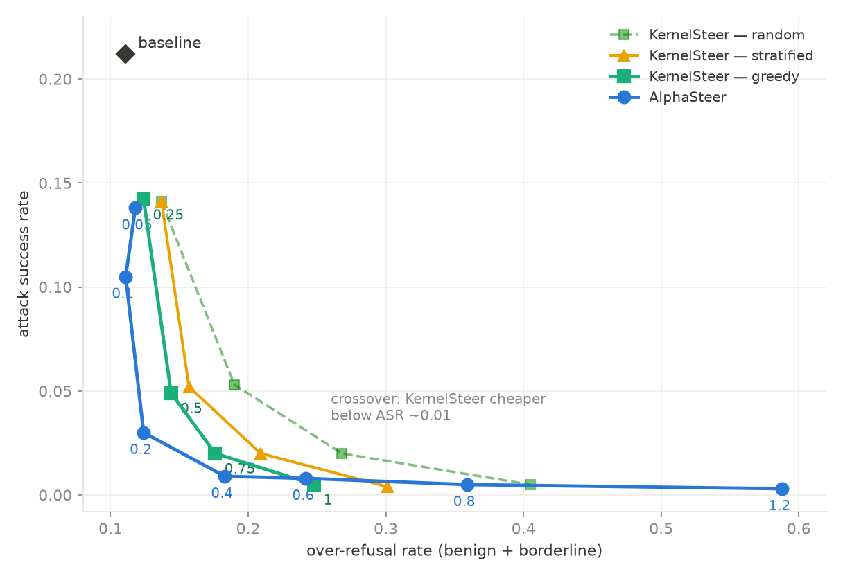
Held-out ASR/ORR frontier; each curve sweeps the steering coefficient. Landmark selection moves KernelSteer’s whole curve left, yet barely underperforms against AlphaSteer.
All KernelSteer results here use m = 1{,}024 landmarks against a fit pool of N = 20{,}386, so the gate is far from the m = N memorization limit. We also swept m from 1,024 to 16,384 at fixed \alpha: ASR was flat and ORR barely changed, hence, tuning m was abandoned.
The same comparison on the training pool tells a different story. In-distribution, greedy KernelSteer dominates: at \alpha = 0.75 it reaches ASR 0.005 at ORR 0.117, which is strictly better than AlphaSteer’s most aggressive point.
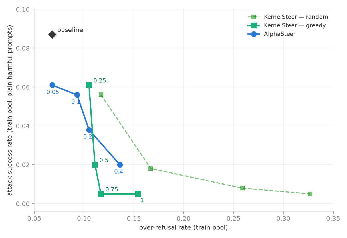
The same comparison on the training pool: greedy KernelSteer at \alpha = 0.75 strictly dominates AlphaSteer’s aggressive end in-distribution.
While this shows promise for KernelSteer’s expressivity over AlphaSteer, the worse performance on the held-out set indicates a generalization problem rooted in the method’s non-parametric nature: the gate scores distance to the landmark sample, so it over-relies on the landmarks having coverage of even slightly out-of-distribution data. The gate cannot tell reconstruction error apart from genuine harmfulness. On the other hand, AlphaSteer’s parametric subspace projection has no such sample-anchoring, which is likely why it generalizes better.
Next steps
I believe this method has some promise although there are some clear limitations regarding the gate. I will be spending some more time rethinking this part of the method, particularly the gate calibration step and see if any progress can be made regarding pushing performance against AlphaSteer. If we can find something, I will run more experiments on different models and against different steering methods in addition to AlphaSteer, then we will likely be able to make an interesting paper. If it does feel like a dead end, however, I’ll start researching some alternative steering approaches.
This calibration step is the part of the method I’m most unsure about and is where I think there is the most room for improvement. ↩︎